A circuit with a single diode and an RL load is shown above. The source vs is an alternating sinusoidal source. If vs = E * sin (wt), vs is positive when 0 < wt < p, and vs is negative when p < wt <2p. When vs starts becoming positive, the diode starts conducting and the positive source keeps the diode in conduction till wt reaches p radians. At that instant defined by wt = p radians, the current through the circuit is not zero and there is some energy stored in the inductor. The voltage across an inductor is positive when the current through it is increasing and it becomes negative when the current through it tends to fall. When the voltage across the inductor is negative, it is in such a direction as to forward-bias the diode. The polarity of voltage across the inductor is as shown in the sketches shown below.
When vs changes from a positive to a negative value, there is current through the load at the instant wt = p radians and the diode continues to conduct till the energy stored in the inductor becomes zero. After that the current tends to flow in the reverse direction and the diode blocks conduction. The entire applied voltage now appears across the diode.
An expression for the current through the diode can be obtained as shown below. It is assumed that the current flows for 0 < wt < b, where b > p . When the diode conducts, the driving function for the differential equation is the sinusoidal function defining the source voltage. During the period defined by b < wt < 2p, the diode blocks current and acts as an open switch. For this period, there is no equation defining the behaviour of the circuit. For 0 < wt < b , the equation (1) defined below applies.

Given a linear differential equation, the solution is found out in two parts. The homogeneous equation is defined by equation (2). It is preferable to express the equation in terms of the angle q instead of 't'. Since q = wt, we get that dq = w.dt. Then equation (2) then gets converted to equation (3). Equation (4) shown above is the solution to this homogeneous equation and is called the complementary integral.
The value of constant A in the complimentary solution is to be evaluated later.
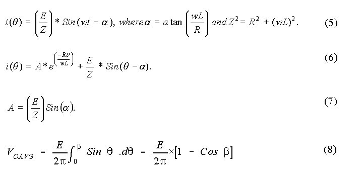
The particular solution is the steady-state response and
equation (5) expresses the particular solution.
The steady-state response is the current that would flow in steady-state
in a circuit that contains only the source, the resistor and the inductor
shown in the circuit above, the only element missing being the diode. This
response can be obtained using the differential equation or the Laplace
transform or the ac sinusoidal circuit analysis. The
total solution is the sum of both the complimentary and the particular
solution and it is shown as equation (6). The value of A is obtained using
the initial condition. Since the diode starts conducting at wt =
0 and the current starts building up from zero, i(0) = 0. The value
of A is expressed by equation (7).
Once the value of A is known, the expression for current is known. After evaluating A, current can be evaluated at different values of wt, starting from wt = p. As wt increases, the current would keep decreasing. For some value of wt, say b , the current would be zero. If wt > b , the current would evaluate to a negative value. Since the diode blocks current in the reverse direction, the diode stops conducting when wt reaches b. Then an expression for the average output voltage can be obtained. Since the average voltage across the inductor has to be zero, the average voltage across the resistor and the average voltage at the cathode of the diode are the same. This average value can be obtained as shown in equation (8).
The operation of the circuit can be simulated as shown below. In order to simulate, the solution for current is presented in the following form, where t = (wL)/R. Then
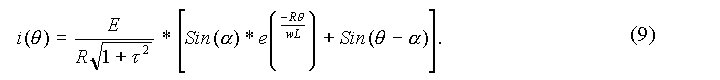
Again it is preferable to normalize. Here E is set to unity and E/R is also set to unity. Then
vs = sin (wt).
vo = i for 0 < wt < b,
vL = vs - i for 0 < wt < b .
To solve the expression, all we need to know is then the ratio t. The applet shown below simulates this circuit. You have to key-in the ratio t and then click on the button next to it. Do not key-in a NaN.
The next page presents the same circuit with an additional diode.
For simulation using Pspice, the circuit used is shown below. Here the nodes are numbered. The ac source is connected between nodes 1 and 0. The diode is connected between nodes 1 and 2 and the inductor links nodes 2 and 3. The resistor is connected from 3 to the reference node, that is, node 0.

The Pspice program is presented below.
* First Chapter: Half-wave Rectifier with RL Load
* A problem to find the diode current
VIN 1 0 SIN(0 340V 50Hz)
D1 1 2 DNAME
L1 2 3 31.8MH
R1 3 0 10
.MODEL DNAME D(IS=10N N=1 BV=1200 IBV=10E-3 VJ=0.6)
.TRAN 10US 60.0MS 20.0MS 10US
.PROBE
.OPTIONS(ABSTOL=1N RELTOL=.01 VNTOL=1MV)
.END
The diode is described using the MODEL statement. The TRAN statement simulates the transient operation for a period of 60 ms at an interval of 10 ms. The OPTIONS statement sets limits for tolerances. The output can be
The Matlab program used is re-produced below.
% Program to simulate the half-wave rectifier circuit
% Enter the peak voltage, frequency, inductance L in mH and resistor R
disp('Typical value for peak voltage is 340 V')
peakV=input('Enter Peak voltage in Volts>');
disp('Typical value for line frequency is 50 Hz')
freq=input('Enter line frequency in Hz>');
disp('Typical value for Load inductance is 31.8 mH')
L=input('Enter Load inductance in mH>');
disp('Typical value for Load Resistance is 10.0 Ohms')
R=input('Enter Load Resistance in Ohms>');

w=2.0*pi*freq;
X=w*L/1000.0;
if (X<0.001) X=0.001; end;
Z=sqrt(R*R+X*X);
loadAng=atan(X/R);
A=peakV/Z*sin(loadAng);
tauInv=R/X;

for n=1:360;
  theta=n/180.0*pi;
  X(n)=n;
  cur=peakV/Z*sin(theta-loadAng)+A*exp(-tauInv*theta);
  if (cur>0.0)
     Vind(n)=peakV*sin(theta)-R*cur;
     iLoad(n)=cur;
     Vout(n)=peakV*sin(theta);
  else
     Vind(n)=0;
     iLoad(n)=0;
     Vout(n)=0;
  end;
end;

plot(X,iLoad)
title('The diode current')
xlabel('degrees')
ylabel('Amps')
grid
pause

plot(X,Vout)
title('Voltage at cathode')
xlabel('degrees')
ylabel('Volts')
grid
pause

plot(X,Vind)
title('Inductor Voltage')
xlabel('degrees')
ylabel('Volts')
grid
The plots obtained for the typical values mentioned
are shown below.
It can be seen from the waveform of voltage across the inductor is that the area above the x-axis at 0 V is equal to its area below the x-axis. It can be seen that the matlab program is relatively simple.
The simulation of this circuit is in a file called halfrec1.mcd. You can download it by clicking on the image below. You need MathCad program to open this file. If you open this file with MathCad program, you can change the parameters and see how the waveforms of output voltage, diode current and voltage across the inductor.
![]()
Alternatively, you can view the mathcad file by clicking on the image below. Then you see the file in HTML format, but you cannot change the parameters.
![]()
This page has described the circuit of a half-wave rectifier.
It has been simulated using different programs. The next page is
on a half-wave rectifier with a free-wheeling diode.