PSPICE SIMULATION
MATLAB SIMULATION
MATHCAD SIMULATION
The circuit shown above differs from the circuit described in the previous page, which had only diode D1. This circuit has another diode, marked D2 in the circuit shown above. This diode is called the free-wheeling diode. The circuit operation is described next. The explanation is based on the assumption that the reader knows how the circuit without a free-wheeling diode operates.
The difference in solution is in how the constant A in complementary integral is evaluated. In the case of the circuit without free-wheeling diode, i(0) = 0, since the current starts building up from zero at the start of every positive half-cycle. On the other hand, the current-flow is continuous when the circuit contains a free-wheeling diode also. Since the input to the RL circuit is a periodic half-sinusoid function, we expect that the response of the circuit should also be periodic. That means, the current through the load is periodic. It means that i(0) = i(2p).
Since the current through the load free-wheels during p < q < 2p , we get equation (6). We use ( q - p ) for the elapsed period in radians instead of q itself, since the free-wheeling action starts at q = p . From the total solution, we can get i(p) from equation (7) by substituing q = p. To obtain A, the following steps are necessary. From the total solution, obtain an expression for i(0) by substituting 0 for q. Also obtain an expression for i(p) by substituting p for q in equation (7). Using this expression for i(p) in equation (6), obtain i(2p) by letting q = 2p . Since i(0) = i(2p), we can obtain A from equation (8). In equation (8), the terms containing constant A are grouped on the left-hand side of equation and the other terms on the right-hand side.
vL(q ) = vs(q) - R*i(q) , for 0 < q < p and
= - R*i(q) , for p < q < 2p .
vs(q) = E*sin (q).
It is preferable to normalize vs with respect to E and the current with respect to E/R and then the only value required to be known for solving for the current is t. The applet shown below simulates this circuit. You have to key-in the ratio t and then click on the button next to it. Do not key-in a NaN.
The circuit that is used for Pspice simulation is shown below. The nodes are numbered and the components have been labeled.

A Pspice program to simulate the circuit shown above is presented now.
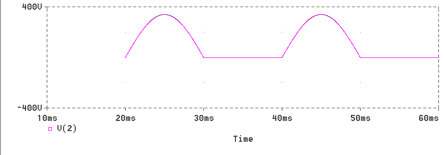
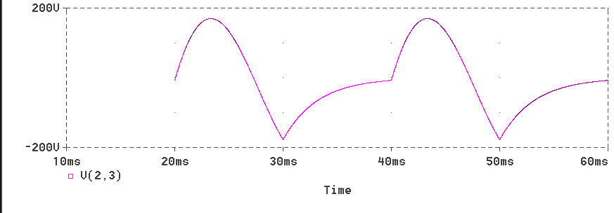
* Half-wave Rectifier with free-wheeling diode and with RL Load
* A problem to find the diode current
VIN 1 0 SIN(0 340V 50Hz)
D1 1 2 DNAME
L1 2 3 31.8MH
R1 3 0 10
D2 0 2 DNAME
.MODEL DNAME D(IS=10N N=1 BV=1200 IBV=10E-3 VJ=0.6)
.TRAN 10US 60.0MS 20.0MS 10US
.PROBE
.OPTIONS(ABSTOL=1N RELTOL=.01 VNTOL=1MV)
.END
The waveforms obtained are presented now. Since the program specifies that the waveforms be displayed from the second cycle, there is no output for the first 20 ms. The waveform of voltage at the cathode of both diodes is shown below.
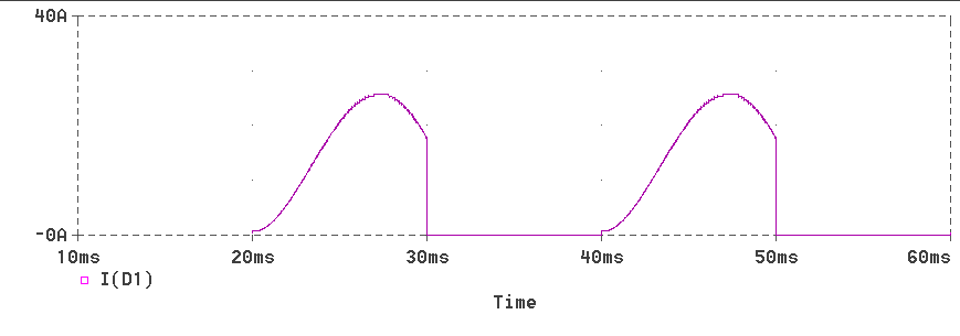
The waveform of current through diode D1 is
presented next.
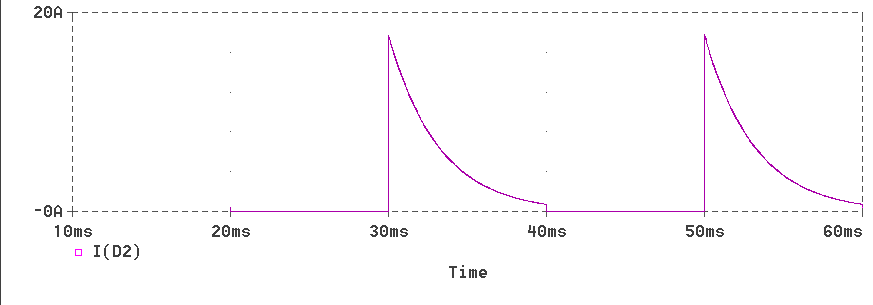
The waveform of current through diode D2 is
shown below.
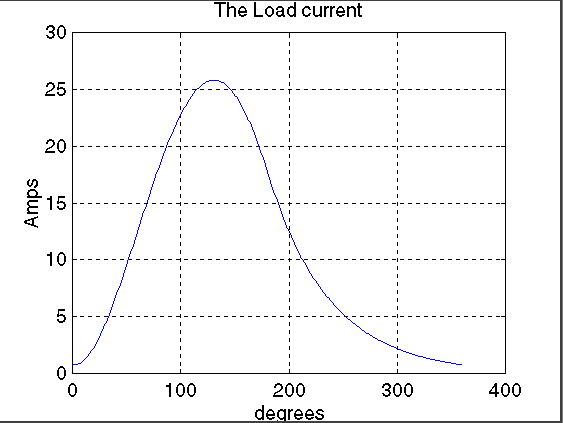
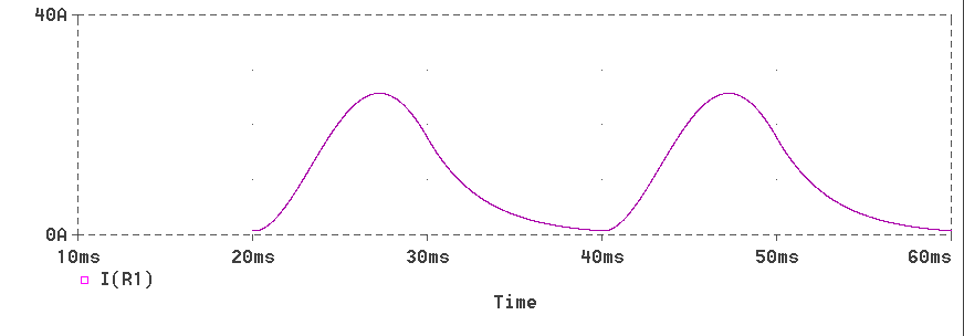
The waveform of current through load resistor is shown
below. It is the sum of both diode currents.
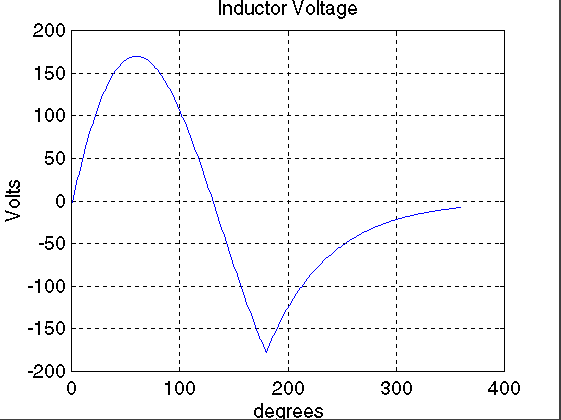
The waveform of voltage across the inductor is shown below.
The advantage with Pspice is the simplicity of the program. In addition, the devices used are also simulated using the spice models.
A matlab program for simulating the half-wave rectifier
with a free-wheeling diode is presented below.
% Program to simulate the half-wave rectifier circuit
% The circuit has a free-wheeling diode
% Enter the peak voltage, frequency, inductance L in mH and resistor R
disp('Typical value for peak voltage is 340 V')
peakV=input('Enter Peak voltage in Volts>');
disp('Typical value for line frequency is 50 Hz')
freq=input('Enter line frequency in Hz>');
disp('Typical value for Load inductance is 31.8 mH')
L=input('Enter Load inductance in mH>');
disp('Typical value for Load Resistance is 10.0 Ohms')
R=input('Enter Load Resistance in Ohms>');
w=2.0*pi*freq;
X=w*L/1000.0;
if (X<0.001) X=0.001; end;
Z=sqrt(R*R+X*X);
tauInv=R/X;
loadAng=atan(X/R);
A1=peakV/Z*sin(loadAng);
A2=peakV/Z*sin(pi-loadAng)*exp(-pi*tauInv);
A3=(A1+A2)/(1-exp(-2.0*pi*tauInv));
Ampavg=0;
AmpRMS=0;
for n=1:360;
theta=n/180.0*pi;
X(n)=n;
if (n<180)
cur=peakV/Z*sin(theta-loadAng)+A3*exp(-tauInv*theta);
Ampavg=Ampavg+cur*1/360;
AmpRMS=AmpRMS+cur*cur*1/360;
else
A4=peakV/Z*sin(pi-loadAng)*exp(-(theta-pi)*tauInv);
cur=A4+A3*exp(-tauInv*theta);
Ampavg=Ampavg+cur*1/360;
AmpRMS=AmpRMS+cur*cur*1/360;
end;
if (n<180)
Vind(n)=peakV*sin(theta)-R*cur;
Vout(n)=peakV*sin(theta);
diode2cur(n)=0;
diode1cur(n)=cur;
else
Vind(n)=-R*cur;
Vout(n)=0;
diode2cur(n)=cur;
diode1cur(n)=0;
end
iLoad(n)=cur;
end;
plot(X,iLoad)
title('The Load current')
xlabel('degrees')
ylabel('Amps')
grid
pause
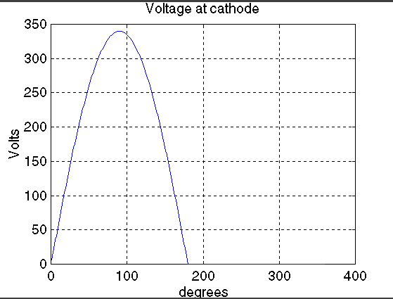
plot(X,Vout)
title('Voltage at cathode')
xlabel('degrees')
ylabel('Volts')
grid
pause
plot(X,Vind)
title('Inductor Voltage')
xlabel('degrees')
ylabel('Volts')
grid
pause
plot(X,diode1cur)
title('Diode 1 current')
xlabel('degrees')
ylabel('Amps')
grid
pause
plot(X,diode2cur)
title('Diode 2 current')
xlabel('degrees')
ylabel('Amps')
grid
AmpRMS=sqrt(AmpRMS);
[A,message]=fopen('outhfr2.dat','w');
fprintf(A,'Avg Load Cur=\t%d\tRMS Load Cur=\t%f\n',Ampavg,AmpRMS);
fclose(A)
The responses obtained for the typical specified values are
shown below.
The average and rms values of load current are presented below.
Avg Load Cur= 1.082254e+001 RMS Load Cur= 13.954542MATHCAD SIMULATION
This circuit can be simulated using MathCad as shown next.
Click on DOWNLOAD to download the file containing the program and then
open it using MathCad. Click on VIEW ONLY to view this file in HTML
format.
![]()
![]()
It has been shown how the half-wave rectifier with a free-wheeling
diode can be simulated using different
software packages. The next page shows how a half-wave
controlled rectifier circuit operates.