This chapter describes the operation of a single-phase fully- controlled bridge rectifier circuit with a load consisting of both resistance and inductance. In addition, the inductance of ac source supplying power to the circuit is taken into account.
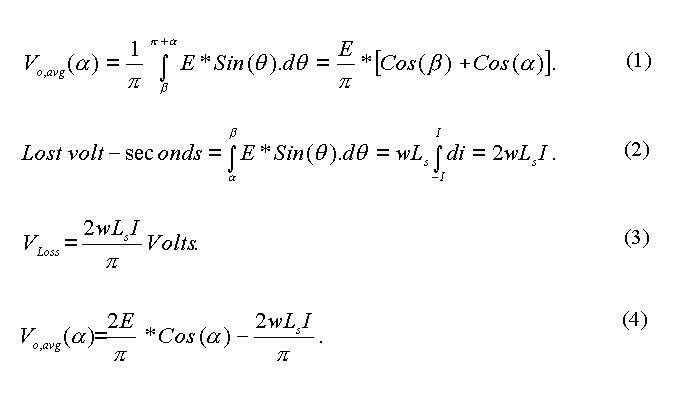
Since this area is lost over p radians, the average value of output voltage lost due to commutation is calculated as shown in equation (3). It is known that the average output voltage with no commutation overlap is (2E/p)*Cos (a). By subtracting the voltage lost due to commutation, we can get the average output voltage taking into account the effect of commutation overlap, as shown in equation (4).


The next applet displays the transient response of the load current. If the load inductance is large, the transient response may last for a few cycles before it settles down to a periodic response. The load current starts building up from zero from the instant one of the pairs of SCRs is triggered first. The response shown starts from this instant.
The next applet shows how the average bridge output voltage,
the rms output voltage, and the ripple factor vary with firing angle for
a given set of wLL/RL and wLs/RL.
This program may take some time to run.

* Full-wave Bridge Rectifier with RL Load and source Inductance
VIN 9 0 SIN(0 340V 50Hz)
XT1 1 2 5 2 SCR
XT2 0 2 6 2 SCR
XT3 4 0 7 0 SCR
XT4 4 1 8 1 SCR
VP1 5 2 PULSE(0 10 1667U 1N 1N 100U 20M)
VP2 6 2 PULSE(0 10 11667U 1N 1N 100U 20M)
VP3 7 0 PULSE(0 10 1667U 1N 1N 100U 20M)
VP4 8 1 PULSE(0 10 11667U 1N 1N 100U 20M)
L1 2 3 31.8M
L2 1 9 1.6M
R1 3 4 10
R2 1 0 1MEG
R3 2 0 1MEG
R4 4 0 1MEG

* Subcircuit for SCR
.SUBCKT SCR 101 102 103 102
S1 101 105 106 102 SMOD
RG 103 104 50
VX 104 102 DC 0
VY 105 107 DC 0
DT 107 102 DMOD
RT 106 102 1
CT 106 102 10U
F1 102 106 POLY(2) VX VY 0 50 11
.MODEL SMOD VSWITCH(RON=0.0105 ROFF=10E+5 VON=0.5 VOFF=0)
.MODEL DMOD D((IS=2.2E-15 BV=1200 TT=0 CJO=0)
.ENDS SCR
.TRAN 10US 60.0MS 0.0MS 10US
.FOUR 50 V(2,4) I(VIN)
.PROBE
.OPTIONS(ABSTOL=1N RELTOL=.01 VNTOL=1MV)
.END
Instead of a Matlab program, a C program is presented below. You can download this file by clicking on the image displayed below. This file, called fcb_1pha.cpp, can be complied just as a C program and no feature of C++ has been used in this program. This program produces an output file called tran_v1.csv and stores in it in the same directory in which the source file is located. This file can be opened by a spreadsheet program like EXCEL and the plots displayed can be obtained.
C Program
// Simulation of a single-phase fully-controlled bridge
// rectifier circuit.
// This program produces the transient response, the periodic
// response. Commuation overlap angle is also computed.
// Calculations normalized.  The average voltage that would
// occur for diode-bridge rectifier with a resistive load is
// taken to be unity.  The average current through the load
// resistor with a pure resistive load on the diode bridge
// rectifier is taken as the unity current.  The parameters to
// be fed are just three: the ratio of load inductive reactance
// to the load resistance, wL1/R , the ratio of source reactance
// to the load resistance to load resistance wL2/R and the firing
// angle in degrees.


#include <math.h>
#include<stdlib.h>
#include<stdio.h>
#include<string.h>
#include<iostream.h>

void kreateRespFile(void);
void tranResponse(void);
void OneCycle(void);
void computeOneStep(void);
void produceEntries(void);


const double pi=3.1415926;
const double deg_rad=pi/180.0;
const double step=pi/720.0;

double L1,L2,alpha,fang,elapseAng,cycleAng,tote_knt;
double cur_load,cur_line,outVolt,vSource,vInput;
double OverLapangle;
int commute,toggle,yes_Entry,modeSw;
FILE *fnew;
char *tstr,*p;


int main(void)
{
 float  ka1,kb2,kc3;
 printf(" \n");
 printf("     Load Time Constant in radians = ");
 scanf("%f",&ka1);
 L1=(double)ka1;
 if (L1<0.05) L1=0.05;
 printf(" \n");
 printf("     Line Reactance Time Constant in radians = ");
 scanf("%f",&kb2);
 L2=(double)kb2;
 printf(" \n");
 printf("     Firing angle in degrees = ");
 scanf("%f",&kc3);
 alpha=(double)kc3;
 fang=alpha*deg_rad;
 alpha=0.0;
 printf("  \n");

 // Initialise though not necessary for global variables

 elapseAng=0.0 ;  cycleAng=0.0;
 cur_load=0.0;  cur_line=0.0;  outVolt=0.0;  tote_knt=0.0;
 OverLapangle=0.0;  commute=0;  yes_Entry=0;


 // Create a file for entering transient response
 fnew=fopen("tran_v1.csv","w+r");
 tranResponse();
 fclose(fnew);
 return 0;
}

void kreateRespFile(void)
{
 int n1,n2;

 tstr="Angle,InputV,VoutBr,LoadCur,LineCur,IndVolt";
 p=strtok(tstr,",");
 fprintf(fnew,p); fprintf(fnew,",");
 n2=6;
 for (n1=0;n1<(n2-1);n1++)
        {
         p=strtok(NULL,",");
         if (n1!=(n2-2))
                {
                 fprintf(fnew,p); fprintf(fnew,",");
                }
         else
                {
                 fprintf(fnew,p); fprintf(fnew,"\n");
                }
        }
}

void tranResponse(void)
{
 double d1;
 int NumCycles,count;
 d1=(6.0*(L1+L2))/(2.0*pi)+0.5;
 NumCycles=(int)d1 + 1;
 kreateRespFile();
 modeSw=1;
 for (count=0;count<=NumCycles;count++)
  OneCycle();
}


void OneCycle(void)
{
 int knt;
 double dknt;
 dknt=0.0;


 for (knt=0;knt<1440;knt++)
        {
         cycleAng=dknt*step;
         vInput=pi/2.0*sin(cycleAng);
         if ((cycleAng<fang) || (cycleAng>(fang+pi)))
                {
                 if (cycleAng<fang) vSource=pi/2.0*sin(cycleAng+pi);
                 else vSource=pi/2.0*sin(cycleAng-pi);
                 toggle=0;
                }
         else
                {
                 vSource=pi/2.0*sin(cycleAng);
                 toggle=1;
                }
         if (modeSw!=toggle)
                {
                 commute=1;
                 if (L2<0.0005) commute=0;
                 modeSw=toggle;
                }
         computeOneStep();
         dknt+=1.0;
        }
}

void computeOneStep(void)
{
 double dLoadI,dLineI;

 switch (commute)
        {
         case 0:
          dLoadI=(vSource-cur_load)/(L1+L2)*step;
          cur_load=cur_load+dLoadI;
          if (cur_load<0.00001) cur_load=0.0;
          if (toggle==0) cur_line=-cur_load;
          else cur_line=cur_load;
          outVolt=cur_load+(vSource-cur_load)*L1/(L1+L2);
         break;

         case 1:
          dLoadI=(0.0-cur_load)/L1*step;
          cur_load=cur_load+dLoadI;
          if (cur_load<0.00001) cur_load=0.0;
          dLineI=vInput/L2*step;
          cur_line=cur_line+dLineI;
          if (toggle==1)
                {
                 if (cur_line>cur_load) commute=0;
                }
          if (toggle==0)
                {
                 if ((cur_line+cur_load)<0.0) commute=0;
                }
          outVolt=0.0;
         break;
        }
 tote_knt+=1.0;
 elapseAng=tote_knt*step;
 alpha=tote_knt/4.0;
 yes_Entry+=1;
 if (yes_Entry==4) produceEntries();
 if (yes_Entry==4) yes_Entry=0;
}

void produceEntries(void)
{
 double negate;
 gcvt(alpha,5,p);
 fprintf(fnew,p);
 fprintf(fnew,",");
 gcvt(vInput,5,p);
 fprintf(fnew,p);
 fprintf(fnew,",");
 gcvt(outVolt,5,p);
 fprintf(fnew,p);
 fprintf(fnew,",");
 gcvt(cur_load,5,p);
 fprintf(fnew,p);
 fprintf(fnew,",");
 gcvt(cur_line,5,p);
 fprintf(fnew,p);
 fprintf(fnew,",");
 if (toggle==0) negate = 1.0; else negate=-1.0;
 gcvt(vInput-negate*outVolt,5,p);
 fprintf(fnew,p);
 fprintf(fnew,"\n");
}
The responses obtained for L1=1.5, L2=0.2 and a = 30o are produced below.
Another C program is presented below. This program carries out the harmonic analysis. This file, called fcb_1phb.cpp, can be downloaded. It can also be compiled as a C program. It produces an output file, called harm_v1.csv.
![]()
C Program
// Simulation of a single-phase fully-controlled bridge
// rectifier circuit.
// This program obtainss the periodic response first
and
// then computes the ripple components in output current
// and voltage and the harmonic components in the line
current.
// The parameters to be fed are just three: the ratio
of load
// inductive reactance to the load resistance, wL1/R
, the
// ratio of source reactance to the load resistance to
load
// resistance wL2/R and the firing angle in degrees.
#include <math.h>
#include<stdlib.h>
#include<stdio.h>
#include<string.h>
void periodicResponse(void);
void harmonicAnalysis(void);
void OneCycle(void);
void computeOneStep(void);
void kreateRespFile(void);
void produceEntries(void);
const double pi=3.1415926;
const double deg_rad=pi/180.0;
const double step=pi/720.0;
double L1,L2,fang,cycleAng;
double cur_load,cur_line,outVolt,vSource,vInput;
double OverLapangle,VoAvg,VoRMS,ILoadAvg,ILoadRMS;
double ILineAvg,ILineRMS,THD,RFVolt,RFCur;
int commute,toggle,modeSw;
double anLoadCur[26],bnLoadCur[26],cnLoadCur[26];
double anLineCur[26],bnLineCur[26],cnLineCur[26];
double anOutVolt[26],bnOutVolt[26],cnOutVolt[26];
FILE *fnew;
char *tstr,*p;
void main(void)
{
float ka1,kb2,kc3;
printf(" \n");
printf(" Load Time Constant
in radians = ");
scanf("%f",&ka1);
L1=(double)ka1;
if (L1<0.05) L1=0.1;
printf(" \n");
printf(" Line Reactance
Time Constant in radians = ");
scanf("%f",&kb2);
L2=(double)kb2;
printf(" \n");
printf(" Firing angle in
degrees = ");
scanf("%f",&kc3);
fang=deg_rad*(double)kc3;
printf(" \n");
// Initialise though not necessary for global variables
cycleAng=0.0;
cur_load=0.0; cur_line=0.0; outVolt=0.0;
OverLapangle=0.0; commute=0; modeSw=0;
toggle=0;
// obtain the transient response.
periodicResponse();
harmonicAnalysis();
printf("Close window by clicking on x button at
top right corner \n");
}
void periodicResponse(void)
{
double startVal;
// Calculate one cycle of response and repeat till
the
// response becomes periodic.
do
{
startVal=cur_load;
OneCycle();
} while (fabs(startVal-cur_load)>0.0005);
}
void OneCycle(void)
{
int knt;
double dknt;
dknt=0.0;
for (knt=0;knt<1440;knt++)
{
cycleAng=dknt*step;
vInput=pi/2.0*sin(cycleAng);
if ((cycleAng<fang)
|| (cycleAng>(fang+pi)))
{
if (cycleAng<fang) vSource=pi/2.0*sin(cycleAng+pi);
else vSource=pi/2.0*sin(cycleAng-pi);
toggle=0;
}
else
{
vSource=pi/2.0*sin(cycleAng);
toggle=1;
}
// To
record commutation overlap, the routine described below is used.
// When
commute is 1, overlap ensues. It is set to to 1 whenever
// a
pair of SCRs is triggered at the set firing agnle. It is resset
// by
the compute_one_step routine when overlap ends. This can be
// checked
from the values of load current and line current.
if (modeSw!=toggle)
{
commute=1;
if (L2<0.0005) commute=0;
modeSw=toggle;
}
computeOneStep();
dknt+=1.0;
}
}
void computeOneStep(void)
{
double dLoadI,dLineI;
switch (commute)
{
case
0:
dLoadI=(vSource-cur_load)/(L1+L2)*step;
cur_load=cur_load+dLoadI;
if (cur_load<0.00001) cur_load=0.0;
if (toggle==0) cur_line=-cur_load;
else cur_line=cur_load;
if (cur_load>0.0) outVolt=cur_load+(vSource-cur_load)*L1/(L1+L2);
else outVolt=0.0;
break;
case
1:
dLoadI=(0.0-cur_load)/L1*step;
cur_load=cur_load+dLoadI;
if (cur_load<0.00001) cur_load=0.0;
dLineI=vInput/L2*step;
cur_line=cur_line+dLineI;
if (toggle==1)
{
if (cur_line>cur_load) commute=0;
}
if (toggle==0)
{
if ((cur_line+cur_load)<0.0) commute=0;
}
outVolt=0.0;
break;
}
}
void harmonicAnalysis(void)
{
int m;
double theta,dblm;
int knt;
double dknt;
dknt=0.0;
for (m=0;m<26;m++)
{
anLoadCur[m]=0.0;
bnLoadCur[m]=0.0; cnLoadCur[m]=0.0;
anLineCur[m]=0.0;
bnLineCur[m]=0.0; cnLineCur[m]=0.0;
anOutVolt[m]=0.0;
bnOutVolt[m]=0.0; cnOutVolt[m]=0.0;
}
OverLapangle=0.0;
ILoadAvg=0.0; ILoadRMS=0.0; RFCur=0.0;
ILineAvg=0.0; ILineRMS=0.0; THD=0.0;
VoAvg=0.0; VoRMS=0.0; RFVolt=0.0;
for (knt=0;knt<720;knt++)
{
cycleAng=dknt*step;
vInput=pi/2.0*sin(cycleAng);
if ((cycleAng<fang)
|| (cycleAng>(fang+pi)))
{
vSource=pi/2.0*sin(cycleAng-pi);
toggle=0;
}
else
{
vSource=pi/2.0*sin(cycleAng);
toggle=1;
}
if (modeSw!=toggle)
{
commute=1;
if (L2<0.0005) commute=0;
modeSw=toggle;
}
computeOneStep();
if ((toggle==1) && (commute==1)) OverLapangle=OverLapangle+step;
dblm=0.0;
for
(m=0;m<13;m++)
{
theta=2.0*dblm*cycleAng;
while (theta>(2.0*pi)) theta=theta-2.0*pi;
anLoadCur[2*m]=anLoadCur[2*m]+cur_load*cos(theta)*step;
bnLoadCur[2*m]=bnLoadCur[2*m]+cur_load*sin(theta)*step;
anOutVolt[2*m]=anOutVolt[2*m]+outVolt*cos(theta)*step;
bnOutVolt[2*m]=bnOutVolt[2*m]+outVolt*sin(theta)*step;
theta=theta+cycleAng;
if (theta>(2.0*pi)) theta=theta-2.0*pi;
anLineCur[2*m+1]=anLineCur[2*m+1]+cur_line*cos(theta)*step;
bnLineCur[2*m+1]=bnLineCur[2*m+1]+cur_line*sin(theta)*step;
dblm=dblm+1.0;
}
ILoadRMS=ILoadRMS+cur_load*cur_load*step;
VoRMS=VoRMS+outVolt*outVolt*step;
ILineAvg=ILineAvg+fabs(cur_line)*step;
ILineRMS=ILineRMS+cur_line*cur_line*step;
dknt+=1.0;
}
for (m=0;m<13;m++)
{
anLoadCur[2*m]=2.0/pi*anLoadCur[2*m];
bnLoadCur[2*m]=2.0/pi*bnLoadCur[2*m];
anOutVolt[2*m]=2.0/pi*anOutVolt[2*m];
bnOutVolt[2*m]=2.0/pi*bnOutVolt[2*m];
anLineCur[2*m+1]=2.0/pi*anLineCur[2*m+1];
bnLineCur[2*m+1]=2.0/pi*bnLineCur[2*m+1];
cnLoadCur[2*m]=anLoadCur[2*m]*anLoadCur[2*m]
+ bnLoadCur[2*m]*bnLoadCur[2*m];
cnLoadCur[2*m]=sqrt(cnLoadCur[2*m]);
cnLineCur[2*m+1]=anLineCur[2*m+1]*anLineCur[2*m+1]
+ bnLineCur[2*m+1]*bnLineCur[2*m+1];
cnLineCur[2*m+1]=sqrt(cnLineCur[2*m+1]);
cnOutVolt[2*m]=anOutVolt[2*m]*anOutVolt[2*m]
+ bnOutVolt[2*m]*bnOutVolt[2*m];
cnOutVolt[2*m]=sqrt(cnOutVolt[2*m]);
}
VoRMS=sqrt(VoRMS/pi);
ILoadRMS=sqrt(ILoadRMS/pi);
ILineAvg= ILineAvg/pi;
ILineRMS= sqrt(ILineRMS/pi);
ILoadAvg=anLoadCur[0]/2.0;
VoAvg=anOutVolt[0]/2.0;
THD=sqrt(ILineRMS*ILineRMS-cnLineCur[0]*cnLineCur[0]/2.0);
RFVolt=sqrt(VoRMS*VoRMS-VoAvg*VoAvg);
RFCur=sqrt(ILoadRMS*ILoadRMS-ILoadAvg*ILoadAvg);
fnew=fopen("harm_v1.csv","w+r");
kreateRespFile();
produceEntries();
fclose(fnew);
}
void kreateRespFile(void)
{
int n1,n2;
tstr="harmNo,LoadCur,OutVolt,harmNo,LineCur";
p=strtok(tstr,",");
fprintf(fnew,p); fprintf(fnew,",");
n2=5;
for (n1=0;n1<(n2-1);n1++)
{
p=strtok(NULL,",");
if (n1!=(n2-2))
{
fprintf(fnew,p); fprintf(fnew,",");
}
else
{
fprintf(fnew,p); fprintf(fnew,"\n");
}
}
}
void produceEntries(void)
{
int m;
for(m=0;m<13;m++)
{
itoa(2*m,
p, 10);
fprintf(fnew,p);
fprintf(fnew,",");
gcvt(cnLoadCur[2*m],5,p);
fprintf(fnew,p);
fprintf(fnew,",");
gcvt(cnOutVolt[2*m],5,p);
fprintf(fnew,p);
fprintf(fnew,",");
itoa(2*m+1,
p, 10);
fprintf(fnew,p);
fprintf(fnew,",");
gcvt(cnLineCur[2*m+1],5,p);
fprintf(fnew,p);
fprintf(fnew,"\n");
}
fprintf(fnew,"\n");
p="LoadIAvg";
fprintf(fnew,p);
fprintf(fnew,",");
gcvt(ILoadAvg,5,p);
fprintf(fnew,p);
fprintf(fnew,"\n");
p="LoadIRMS";
fprintf(fnew,p);
fprintf(fnew,",");
gcvt(ILoadRMS,5,p);
fprintf(fnew,p);
fprintf(fnew,"\n");
p="RFCur";
fprintf(fnew,p);
fprintf(fnew,",");
gcvt(RFCur,5,p);
fprintf(fnew,p);
fprintf(fnew,"\n");
fprintf(fnew,"\n");
p="VoAvg";
fprintf(fnew,p);
fprintf(fnew,",");
gcvt(VoAvg,5,p);
fprintf(fnew,p);
fprintf(fnew,"\n");
p="VoRMS";
fprintf(fnew,p);
fprintf(fnew,",");
gcvt(VoRMS,5,p);
fprintf(fnew,p);
fprintf(fnew,"\n");
p="RFVolt";
fprintf(fnew,p);
fprintf(fnew,",");
gcvt(RFVolt,5,p);
fprintf(fnew,p);
fprintf(fnew,"\n");
fprintf(fnew,"\n");
p="ILineAvg"; fprintf(fnew,p);
fprintf(fnew,",");
gcvt(ILineAvg,5,p);
fprintf(fnew,p);
fprintf(fnew,"\n");
p="ILineRMS";
fprintf(fnew,p);
fprintf(fnew,",");
gcvt(ILineRMS,5,p);
fprintf(fnew,p);
fprintf(fnew,"\n");
p="THD";
fprintf(fnew,p);
fprintf(fnew,",");
gcvt(THD,5,p);
fprintf(fnew,p);
fprintf(fnew,"\n");
fprintf(fnew,"\n");
p="OverLapAngle";
fprintf(fnew,p);
fprintf(fnew,",");
if (OverLapangle>0.0001) OverLapangle=OverLapangle+step/2.0;
gcvt(OverLapangle,5,p);
fprintf(fnew,p);
fprintf(fnew,"\n");
}
The results obtained are presented below.

This page has described how the fully-controlled bridge rectifier circuit behaves when the source has inductance. In the next page, it is decribed how the operation of this circuit changes when it has a filter capacitor.