The circuit of a single-phase fully-controlled bridge rectifier circuit is shown in the figure above. The circuit has four SCRs. It is preferable to state that the circuit has two pairs of SCRs, with S1 and S3 forming one pair and, S2 and S4 the other pair. For this circuit, vs is a sinusoidal voltage source. When it is positive, the SCRs S1 and S3 can be triggered and then current flows from vs through SCR S1, load inductor L, load resistor R, SCR S3 and back into the source. In the next half-cycle, the other pair of SCRs conducts. Even though the direction of current through the source alternates from one half-cycle to the other half-cycle, the current through the load remains unidirectional.
The main purpose of this circuit is to provide a variable dc output voltage, which is brought about by varying the firing angle. Let vs = E sin wt, with 0 < wt < 360o. If wt = 30o when S1 and S3 are triggered, then the firing angle is said to be 30o. In this instance the other pair is triggered when wt= 210o.
The operation of the circuit is illustrated by animating the functioning of this circuit. Key in the firing angle in degrees and click the button. The source voltage, and the bridge output voltage are also displayed. It is assumed here that the load inductance is quite large. The animation is correct only if the firing angle is less than 90o. The programs under simulation section will run correctly for any firing angle.
Analysis by hand is based on the assumption that the load inductance is sufficiently large to keep the load current ripple-free. Programs written for computer simulation are not based on this assumption and they simulate the operation based on the parameter keyed-in.
When the load current is continuous, the average value of the output voltage is obtained as follows. Let the supply voltage be vs = E*Sin (q ), where q varies from 0 to 2p radians. Since the output waveform repeats itself for every half-cycle, the average output voltage is expressed in equation (1) as a function of a, the firing angle.
If the load current is continuous, the r.m.s. value of output voltage is obtained as shown in equation (2).
The maximum average output voltage occurs at a firing
angle of 0o. Let it be Vom. Then
the ripple factor RF(a) is defined as shown in equation (3).
Equations (4) and (5) apply when the conduction is discontinuous.
The variation of average output voltage, r.m.s. output voltage and the ripple factor with the firing angle have been shown below, based on the assumption that the load inductance is large. The plots shown below have been normalized with respect to Vom. For example, when the firing angle is 60o, the average output is shown to be 0.5. It means that the actual average output voltage is 0.5Vom. It can also be seen that when the firing angle is 0o, the r.m.s. output voltage is about 1.1Vom and the ripple factor is about 0.48. The ripple factor increases as the firing angle increases.
If the firing angle is highly retarded or if the load
inductance is not sufficiently large, conduction of load current is not
continuous. Let us consider the positive half-cycle. When q
equals the firing angle, the SCRs S1 and S3 are triggered.
Let the load current start from zero at q = a
and let the load current fall to zero when q = p +
b , before the next pair of SCRs is triggered. It means that b
< a . Then the average output voltage is
computed as shown in equation (4), whereas the r.m.s. output voltage
is computed as shown in equation (5).
The value of b can be found out by iteration, as shown in earlier pages. For the case when the conduction is discontinuous, the plots of the average output voltage, the r.m.s. output voltage and the ripple factor are illustrated below. Key-in the ratio of wL/R, where L is the load inductance, R is the load resistance and w is the angular frequency of the source. In practice this ratio can vary from a low value to about 5. The load angle can be defined to be tan-1(wL/R). When the firing angle is less than the load angle, the conduction is continuous. As explained below, the load current is discontinuous if the firing angle is greater than the load angle.
In this section, the expressions for the load current are first derived. Then an expression for the line current can be obtained. The r.m.s line current, the r.m.s. value of the fundamental of line current, the THD in line current, the frequency spectrum of line current, the frequency spectrum and the ripple content of the bridge output voltage and the frequency spectrum and the ripple content of the voltage across the load resistor are also determined.
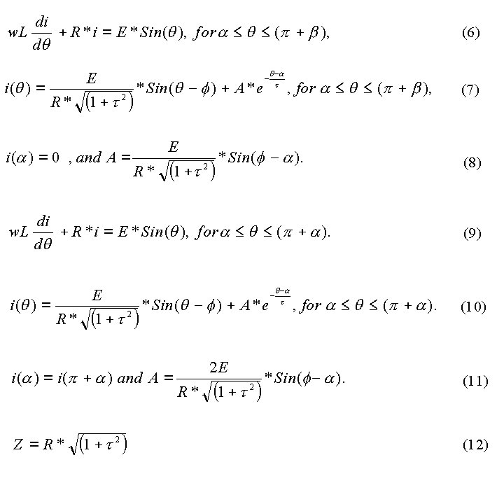
For the case of discontinuous conduction, let the load current in each half cycle flow from q = a till q = p + b , where b < a. During this period, the differential equation that applies to the load current is calculated according to equation (6), where a is the firing angle, (p +b) is the extinction angle and the conduction angle within a cycle is (p + b - a ). The solution to the above equation is obtained as given shown in equation (7). In equation (7), t represents wL/R,the ratio of load reactance to load resistance. f is the load angle, defined to be tan-1(wL/R). When the conduction is discontinuous, the load current starts from zero value at q = a . Hence equation (8) is obtained. When f < a , A has a negative value and we have discontinuous conduction when f < a . It means that the firing of the SCRs is retarded and a > f .
When the conduction is continuous, equation (9) applies.
The solution to equation (9) is presented as equation (10).
Since the signal applied to the load circuit is a periodic
signal, the load current is also periodic, after a transient period. It
means that equation (11) is valid for continuous conduction.
For continuous conduction, f
> a and A is positive. When f
= a, the conduction is about to become continuous
and the value of A should satisfy both expressions for A. It is seen that
f = a, A = 0 according
to both expressions for A. When f = a
, the current drawn from the source is sinusoidal and equals (E/Z)*Sin
(wt - f), where Z is defined as shown in equation
(12).
Once the load current is defined for a half-cycle, the
expression for line current can be obtained. It equals the load current
when SCRs S1 and S3 are conducting and it is the
negative of the load current when the other pair of SCRs is conducting.
Further analysis can be carried out using Fourier series and the DPF and
PF of the line current can be determined.
When the circuit is switched on initially, the load current may settle down to a periodic response after a few output cycles. The time constant of the load is L/R and a time period corresponding to five times the constant should elapse before the load current becomes periodic. For example if the load time constant is 20 ms, a time period of 100 ms should pass before the load current becomes periodic. This time period corresponds to five input voltage cycles at 50 Hz and six input cycles at 60 Hz.
The plots for voltage have been normalized with respect
to Vom, the maximum average output voltage and the plots for
line current with respect to Irms,max, which is 0.707E/R. To
see the periodic response, key-in firing angle in degrees in the box on
the left-hand side and the ratio t in the box
on the right-hand side and then click start button. The boxes have default
values filled-in.
The statistical details related to the output voltage
have been normalized with respect to Vom and those related to
the source current with respect to Irms,max. The amplitude of
each harmonic in the output voltage has been normalized with respect to
E which is the amplitude of the source voltage , whereas the amplitude
of each harmonics in the source current has been normalized with respect
to E/R. The applet to follow displays the statistical details.
The applet below displays the transient response.
As the ratio gets larger and larger, the load current requires larger period
to elapse before it becomes periodic.

The program is presented below.
* Full-wave Bridge Rectifier with a resistive load
VIN 1 0 SIN(0 340V 50Hz)
XT1 1 2 5 2 SCR
XT2 0 2 6 2 SCR
XT3 4 0 7 0 SCR
XT4 4 1 8 1 SCR
VP1 5 2 PULSE(0 10 1667U 1N 1N 100U 20M)
VP2 6 2 PULSE(0 10 11667U 1N 1N 100U 20M)
VP3 7 0 PULSE(0 10 1667U 1N 1N 100U 20M)
VP4 8 1 PULSE(0 10 11667U 1N 1N 100U 20M)
L1 2 3 31.8M
R1 3 4 10
R2 1 0 1MEG
R3 2 0 1MEG
R4 4 0 1MEG

* Subcircuit for SCR
.SUBCKT SCR 101 102 103 102
S1 101 105 106 102 SMOD
RG 103 104 50
VX 104 102 DC 0
VY 105 107 DC 0
DT 107 102 DMOD
RT 106 102 1
CT 106 102 10U
F1 102 106 POLY(2) VX VY 0 50 11
.MODEL SMOD VSWITCH(RON=0.0105 ROFF=10E+5 VON=0.5 VOFF=0)
.MODEL DMOD D((IS=2.2E-15 BV=1200 TT=0 CJO=0)
.ENDS SCR
.TRAN 10US 60.0MS 0.0MS 10US
.FOUR 50 V(2,4) I(VIN)
.PROBE
.OPTIONS(ABSTOL=1N RELTOL=.01 VNTOL=1MV)
.END
The responses obtained are shown below.

The Matlab program is presented below.
% Program to simulate the full-wave fully-controlled bridge rectifier
% Simulation at a specified firing angle
% Enter the peak voltage, frequency, inductance L in mH and resistor R
disp('Typical value for peak voltage is 340 V')
peakV=input('Enter Peak voltage in Volts>');
disp('Typical value for line frequency is 50 Hz')
freq=input('Enter line frequency in Hz>');
disp('Typical value for Load inductance is 31.8 mH')
L=input('Enter Load inductance in mH>');
disp('Typical value for Load Resistance is 10.0 Ohms')
R=input('Enter Load Resistance in Ohms>');
disp('Typical value for Firing angle is 30.0 degree')
fangDeg=input('Enter Firing angle within range 0 to 180 in deg>');
fangRad=fangDeg/180.0*pi;

w=2.0*pi*freq;
X=w*L/1000.0;
if (X<0.001) X=0.001; end;
Z=sqrt(R*R+X*X);
tauInv=R/X;
loadAng=atan(X/R);
k1=peakV/Z;
k2=2.0*k1*sin(loadAng-fangRad)/(1.0-exp(-pi*tauInv));
k3=k1*sin(loadAng-fangRad);
if (fangRad<loadAng)
  A=k2;
  sw=1;
else
  A=k3;
  sw=2;
end;

Ampavg=0;
AmpRMS=0;

for n=1:360;
  theta=n/180.0*pi;
  X(n)=n;
  if (sw==1);
    if (n<fangDeg);
          cur=k1*sin(pi+theta-loadAng)+A*exp(-tauInv*(pi+theta-fangRad));
          vbr(n)=peakV*sin(theta+pi);
          vind(n)=vbr(n)-R*cur;
          iLoad(n)=cur;
          vSCR(n)=peakV*sin(theta);
          Ampavg=Ampavg+cur*1/360;
          AmpRMS=AmpRMS+cur*cur*1/360;
        elseif ((n>=fangDeg) & (n<(180+fangDeg)));
          cur=k1*sin(theta-loadAng)+A*exp(-tauInv*(theta-fangRad));
          vbr(n)=peakV*sin(theta);
          vind(n)=vbr(n)-R*cur;
          iLoad(n)=cur;
          vSCR(n)=0;
          Ampavg=Ampavg+cur*1/360;
          AmpRMS=AmpRMS+cur*cur*1/360;
        else (n>=(180+fangDeg));
      cur=k1*sin(theta-pi-loadAng)+A*exp(-tauInv*(theta-pi-fangRad));
          vbr(n)=peakV*sin(theta-pi);
          vind(n)=vbr(n)-R*cur;
          iLoad(n)=cur;
          vSCR(n)=peakV*sin(theta);
          Ampavg=Ampavg+cur*1/360;
          AmpRMS=AmpRMS+cur*cur*1/360;
         end;

  else
    if (n<fangDeg);
          cur=k1*sin(pi+theta-loadAng)+A*exp(-tauInv*(pi+theta-fangRad));
          if (cur>0);
            vbr(n)=peakV*sin(theta+pi);
            vind(n)=vbr(n)-R*cur;
            iLoad(n)=cur;
            vSCR(n)=peakV*sin(theta);
            Ampavg=Ampavg+cur*1/360;
            AmpRMS=AmpRMS+cur*cur*1/360;
          else;
            vbr(n)=0.0;
                vind(n)=0.0;
                iLoad(n)=0.0;
            vSCR(n)=peakV*sin(theta)/2.0;
          end;

        elseif ((n>=fangDeg) & (n<(180+fangDeg)));
          cur=k1*sin(theta-loadAng)+A*exp(-tauInv*(theta-fangRad));
          if (cur>0);
            vbr(n)=peakV*sin(theta);
            vind(n)=vbr(n)-R*cur;
            iLoad(n)=cur;
            vSCR(n)=0;
            Ampavg=Ampavg+cur*1/360;
            AmpRMS=AmpRMS+cur*cur*1/360;
      else;
            vbr(n)=0.0;
                vind(n)=0.0;
                iLoad(n)=0.0;
            vSCR(n)=peakV*sin(theta)/2.0;
          end;

        else (n>=(180+fangDeg));
      cur=k1*sin(theta-pi-loadAng)+A*exp(-tauInv*(theta-pi-fangRad));
          vbr(n)=peakV*sin(theta-pi);
          vind(n)=vbr(n)-R*cur;
          iLoad(n)=cur;
          vSCR(n)=peakV*sin(theta);
          Ampavg=Ampavg+cur*1/360;
          AmpRMS=AmpRMS+cur*cur*1/360;
        end;
  end;
end;


plot(X,iLoad)
title('The Load current')
xlabel('degrees')
ylabel('Amps')
grid
pause

plot(X,vbr)
title('Bridge Output volt')
xlabel('degrees')
ylabel('Volts')
grid
pause

plot(X,vind)
title('Inductor Voltage')
xlabel('degrees')
ylabel('Volts')
grid
pause

plot(X,vSCR)
title('SCR Voltage')
xlabel('degrees')
ylabel('Volts')
grid


AmpRMS=sqrt(AmpRMS);
[C,message]=fopen('fwrl1ph1.dat','w');
fprintf(C,'Avg Load Cur=\t%d\tRMS Load Cur=\t%f\n',Ampavg,AmpRMS);
fclose(C);
The responses obtained for the typical specified values have
been displayed below.

The results obtained with a firing angle of 60o have been displayed below. The other values are the same as for the previous set. When the firing angle is retarded this much, the load current is discontinuous.

This page has described the operation of a fully-controlled bridge rectifier circuit with an RL load. Even though the circuit has been simulated using Pspice, Mathcad and Matlab, it is difficult to reach the level of interactive programming that can be achieved with Java or C by using these packages. Next page describes the operation of this circuit when the source inductance is also taken into account.